In a previous post, we demonstrated how to use Hue's Search app to seamlessly index and visualize trip data from Bay Area Bike Share and use Spark to supplement that analysis by adding weather data to our dashboard.
In this tutorial, we'll use the Notebook app to study deeper the peak usage of the Bay Area Bike Share (BABS) system.
To start, download the latest data set from ( http://www.bayareabikeshare.com/datachallenge</a></del> the original website doesn't have the data anymore) https://github.com/evizitei/BikeShareAnalysis. This post uses the data from August 2013 through February 2014.
The notebook can be downloaded here and imported like workflows or search dashboard.
https://www.youtube.com/watch?v=tcdGNOBLelQ
Importing CSV Data with the Metastore App
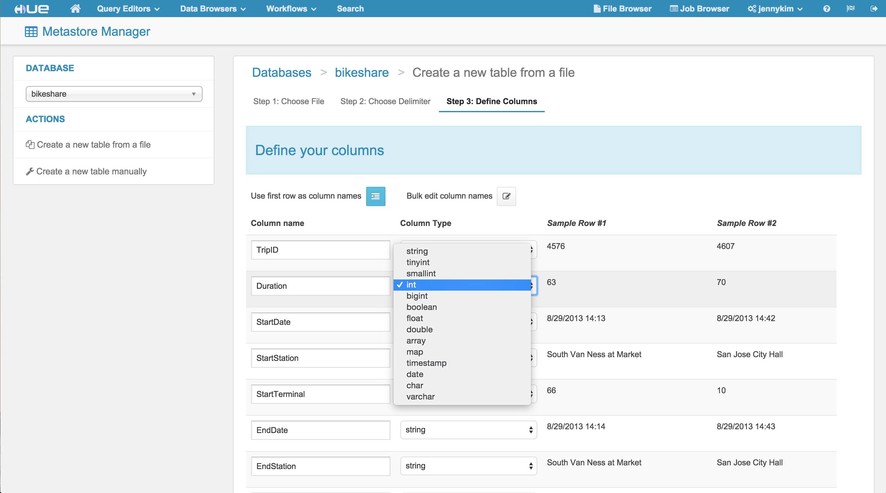
The BABS data set contains 4 CSVs that contain data for stations, trips, rebalancing (availability), and weather. Using Hue's Metastore import wizard, we can easily import these data sets and create tables that infer their schema from the CSV header.
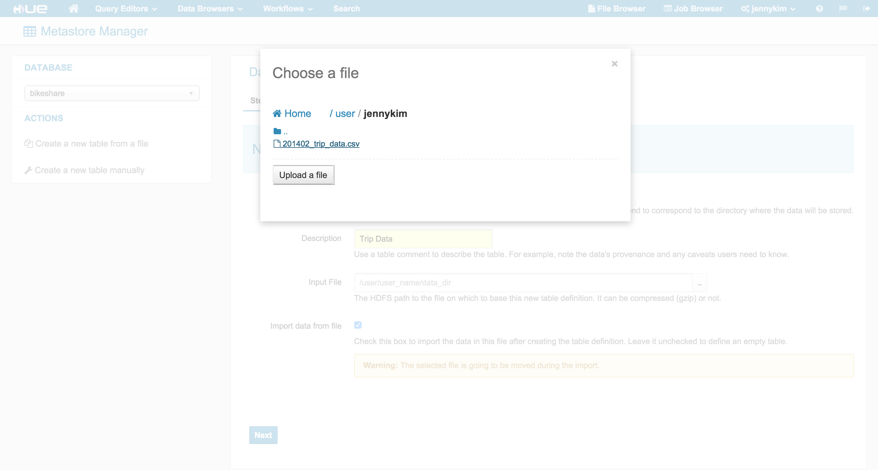
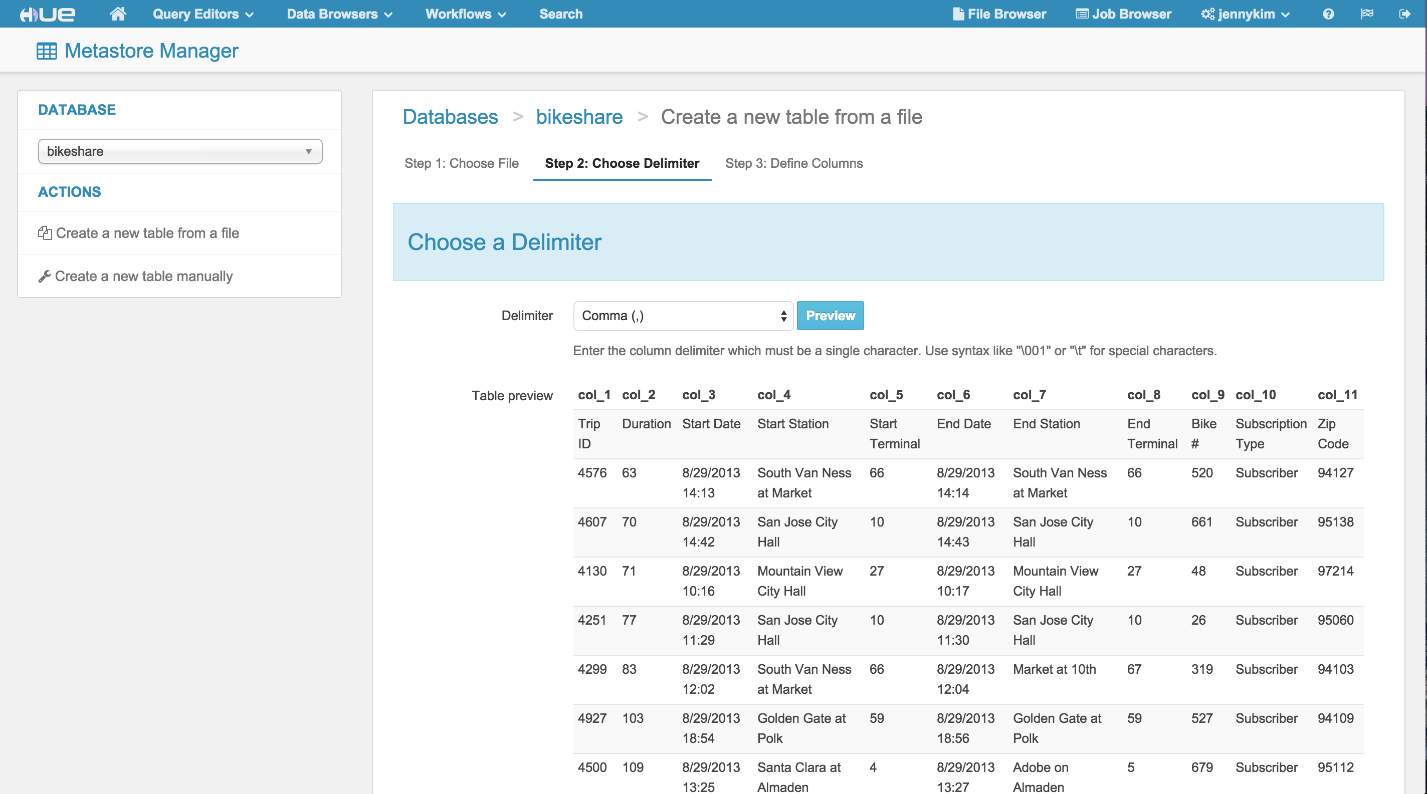
The import wizard also provides the opportunity to override any field names or types, which we'll do for the Trip data to change the “duration” field from a TINYINT to an INT.
Interactive Analysis with an Hadoop Notebook
Lightning-Fast Impala Queries
Now that we've imported the data into our cluster, we can create a new Notebook to perform our data crunching. To start, we'll run some quick exploration queries using Impala.
Let's find the top 10 most popular start stations based on the trip data:
SELECT startterminal, startstation, COUNT(1) AS count FROM bikeshare.trips GROUP BY startterminal, startstation ORDER BY count DESC LIMIT 10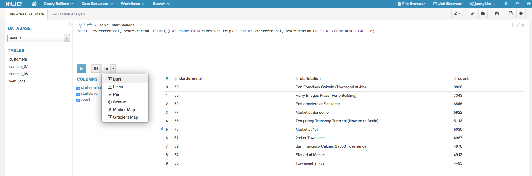
Once our results are returned, we can easily visualize this data; a bar graph works nicely for a simple COUNT..GROUP BY query.

It seems that the San Francisco Caltrain (Townsend at 4th) was by far the most common start station. Let's determine which end stations, for trips starting from the SF Caltrain Townsend station, were the most popular. We'll fetch the latitude and longitude coordinates so that we can visualize the results on a map.
SELECT

s.station_id,

s.name,

s.lat,

s.long,

COUNT(1) AS count

FROM \`bikeshare\`.\`trips\` t

JOIN \`bikeshare\`.\`stations\` s ON s.station_id = t.endterminal

WHERE t.startterminal = 70

GROUP BY s.station_id, s.name, s.lat, s.long

ORDER BY count DESC LIMIT 10
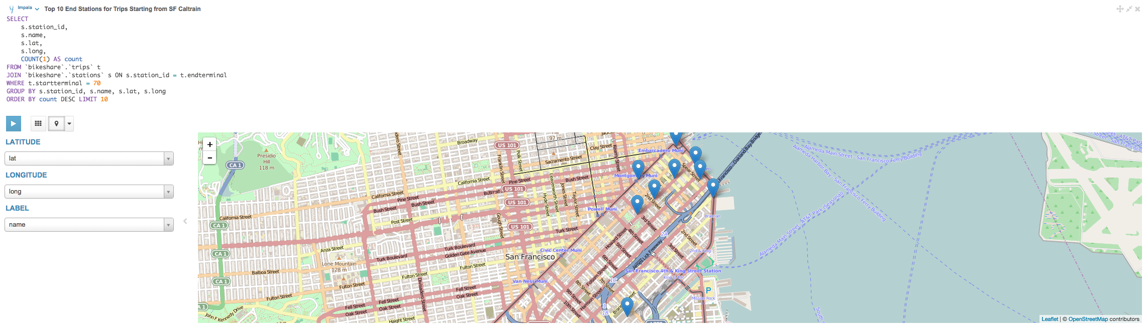
The map visualization indicates that the most popular trips starting from the SF Caltrain station are in fairly close proximity to the station, with most of the destinations being clustered around the Financial District and SOMA.
Long Running Queries with Hive
For longer-running SQL queries, or queries that require use of Hive's built-in functions, we can add a Hive snippet to our notebook to perform this analysis.
Let's say we wanted to dig further into the trip data for the SF Caltrain station and find the total number of trips and average duration (in minutes) of those trips, grouped by hour.
Since the trip data stores startdate as a STRING, we'll need to apply some string-manipulation to extract the hour within an inline SQL query. The outer query will aggregate the count of trips and the average duration.
SELECT

hour,

COUNT(1) AS trips,

ROUND(AVG(duration) / 60) AS avg_duration

FROM (

SELECT

CAST(SPLIT(SPLIT(t.startdate, ' ')[1], ':')[0] AS INT) AS hour,

t.duration AS duration

FROM \`bikeshare\`.\`trips\` t

WHERE

t.startterminal = 70

AND

t.duration IS NOT NULL

) r

GROUP BY hour

ORDER BY hour ASC;
Since this data produces several numeric dimensions of data, we can visualize the results using a scatterplot graph, with the hour as the x-axis, number of trips as the y-axis, and the average duration as the scatterplot size.

Let's add another Hive snippet to analyze an hour-by-hour breakdown of availability at the SF Caltrain Station:
SELECT

hour,

ROUND(AVG(bikes_available)) AS avg_bikes,

ROUND(AVG(docks_available)) AS avg_docks

FROM (

SELECT

r.time AS time,

CAST(SUBSTR(r.time, 12, 2) AS INT) AS hour,

CAST(r.bikes_available AS INT) AS bikes_available,

CAST(r.docks_available AS INT) AS docks_available

FROM \`bikeshare\`.\`rebalancing\` r

JOIN \`bikeshare\`.\`stations\` s ON r.station_id = s.station_id

WHERE

r.station_id = 70

AND

SUBSTR(r.time, 15, 2) = '00'

) t

GROUP BY hour

ORDER BY hour ASC;
We'll visualize the results as a line graph, which indicates that the bike availability tends to fall starting at 6 AM and is regained around 6 PM.

Robust Data Analysis with PySpark
At a certain point, your data analysis may exceed the limits of relational analysis with SQL or require a more expressive, full-fledged API.
Hue's Spark notebooks allow users to mix exploratory SQL-analysis with custom Scala, Python (pyspark), and R code that utilizes the Spark API.
For example, we can open a pyspark snippet and load the trip data directly from the Hive warehouse and apply a sequence of filter, map, and reduceByKey operations to determine the average number of trips starting from the SF Caltrain Station:
trips = sc.textFile('/user/hive/warehouse/bikeshare.db/trips/201402_trip_data.csv')

trips = trips.map(lambda line: line.split(","))

station_70 = trips.filter(lambda x: x[4] == '70')

\# Emit tuple of ((date, hour), 1)

trips_by_day_hour = station_70.map(lambda x: ((x[2].split()[0], x[2].split()[1].split(':')[0]), 1))

trips_by_day_hour = trips_by_day_hour.reduceByKey(lambda a, b: a+b)

\# Emit tuple of (hour, count)

trips_by_hour = trips_by_day_hour.map(lambda x: (int(x[0][1]), x[1]))

avg_trips_by_hour = trips_by_hour.combineByKey( (lambda x: (x, 1)),

(lambda x, y: (x[0] + y, x[1] + 1)),

(lambda x, y: (x[0] + y[0], x[1] + y[1]))

)

avg_trips_by_hour = avg_trips_by_hour.mapValues(lambda v : v[0] / v[1])

avg_trips_sorted = sorted(avg_trips_by_hour.collect())

%table avg_trips_sorted
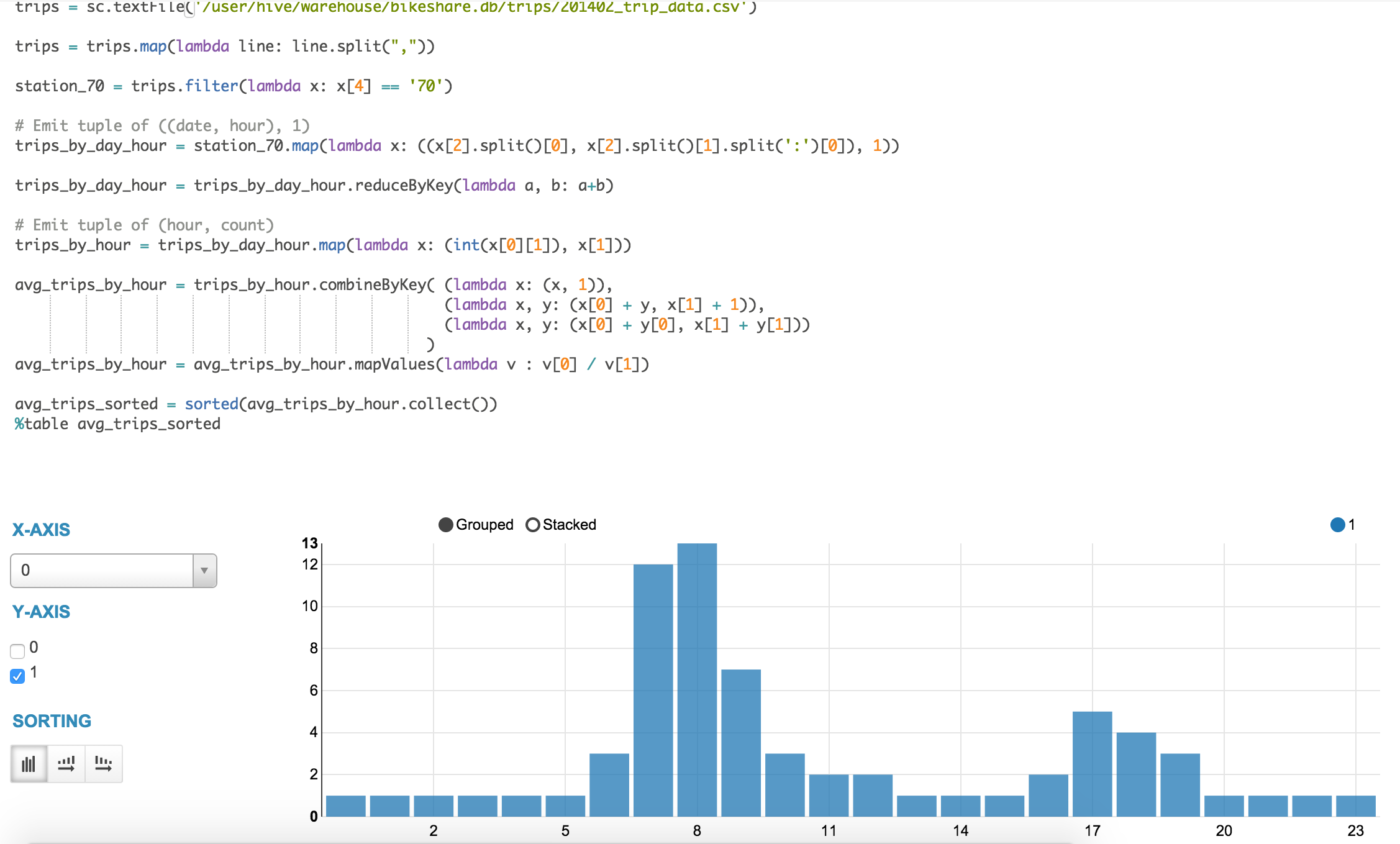
As you can see, Hue's Notebook app enables easy interactive data analysis and visualizations with a powerful mix of tools. Want to know more about the Spark Notebook work, read about the Livy, the Spark REST Job server and see you at the upcoming Hadoop World in New York and Spark Summit in Amsterdam!
Stay tuned for a number of exciting improvements to the notebook app, and as usual feel free to comment on the hue-user list or @gethue!
Helpful Tips
Importing quoted-CSV data
The BABS rebalancing data (named 201402_status_data.csv) uses quotes. In these cases, it is easier to create the table in Hive in the Beeswax editor and use the OpenCSV Row SERDE for Hive:
CREATE TABLE rebalancing(station_id int, bikes_available int, docks_available int, time string)

ROW FORMAT SERDE 'org.apache.hadoop.hive.serde2.OpenCSVSerde'

WITH SERDEPROPERTIES (

"separatorChar" = ",",

"quoteChar" = "\"",

"escapeChar" = "\\"

)

STORED AS TEXTFILE;
Then you can go back to the Metastore to import the CSV into the table; note that you may have to remove the header line manually.
Reset Impala's Metastore Cache
When you create new databases or tables and plan to query them in an Impala snippet, it's a good idea to run an INVALIDATE METADATA; command first to reset the metastore cache. Otherwise, you may encounter an error where the database or table is not recognized.